Monte Carlo simulation: what it is and where MetisTrades uses it
A Monte Carlo simulation replays an uncertain future thousands of times and reports the spread instead of one number. Learn to run a small one by hand from your own closed trades, then see the three places MetisTrades runs one for you.
What it is and why it matters
A Monte Carlo simulation is a way of answering a question about the future when you cannot know the answer: you replay the future many thousands of times with the uncertain parts drawn at random, then look at the whole collection of results rather than any single one.
That last part is the point. A single projection — "my average trade makes $22, so 50 trades should make about $1,100" — is one line through a cloud of possibilities. It tells you nothing about how bumpy the ride is, how often the year ends red, or how deep the worst stretch gets. A simulation keeps the cloud.
Two words you will meet throughout. A run (also called a path) is one simulated future: one possible sequence of trades, or one possible price path. A percentile is a position in the sorted list of results: the 10th percentile is the value that 1 run in 10 falls below, and the 90th is the value that 1 run in 10 exceeds. The gap between them is the band most of your outcomes live in.
What gets drawn at random is the design decision that defines each simulation. There are two common choices:
- Bootstrap (resampling) — draw from outcomes that actually happened to you. Every simulated trade is one of your real closed trades, picked at random with replacement, so the same trade can be picked twice in one run. The method invents no new outcomes, only new orderings and frequencies.
- Model-based paths — draw from a mathematical model of prices, such as a lognormal return at a chosen volatility, then reprice your positions at the end of each path.
Neither is a forecast. A bootstrap assumes your future trades resemble your past ones; a price model assumes the shape and size of moves you fed it. Both are honest about one thing a point estimate hides: the spread. That is why traders use them — to see how often a perfectly reasonable strategy still produces a losing stretch, and how deep that stretch can go.
How to track it by hand
You can run a usable Monte Carlo with a 10-sided die and two sheets of paper. The worked example below bootstraps ten closed trades into ten simulated futures of five trades each.
Step 1: list the outcomes the simulation may draw from
Start with your closed trades, numbered 1 upward. Treat a whole roll chain as one trade — if you rolled a short put three times before closing it, that is one outcome, not four, because the rolls were never independent decisions. Record the exit date, the symbol and the net profit or loss.
| # | Closed | Symbol | P/L | Win (1/0) |
|---|---|---|---|---|
| 1 | 2026-01-09 | XYZ | 120 | 1 |
| 2 | 2026-01-16 | ABC | 95 | 1 |
| 3 | 2026-01-23 | DEF | 110 | 1 |
| 4 | 2026-01-30 | XYZ | -480 | 0 |
| 5 | 2026-02-06 | ABC | 130 | 1 |
| 6 | 2026-02-13 | DEF | 85 | 1 |
| 7 | 2026-02-20 | XYZ | 105 | 1 |
| 8 | 2026-02-27 | ABC | -150 | 0 |
| 9 | 2026-03-06 | DEF | 90 | 1 |
| 10 | 2026-03-13 | XYZ | 115 | 1 |
Eight of the ten made money, so the win rate is 0.8. The ten results add to 220, which is an average of 22 per trade. On its own that record looks tidy: four wins in five, and a positive expectancy.
Step 2: draw five trades at random, with replacement
Roll a 10-sided die five times. Each roll picks a trade number from the list above, and you put the number back each time, so trade 4 can appear twice in one run and not at all in the next. Write down the five picks, look up each one's P/L, and add them. That total is one possible future.
Run 1 drew 6, 3, 6, 10, 7. Trade 6 came up twice. The P/L values are 85, 110, 85, 115 and 105, which total 500 — no losers drawn, so the run is strongly positive. Run 3 drew 3, 2, 10, 1, 4: 110 + 95 + 115 + 120 − 480 = −40. Four winners and one −480 loser is enough to put the run in the red. Run 9 drew the −480 twice and the −150 once: −480 + 110 − 150 − 480 + 90 = −910.
Step 3: do it ten times and read the spread
| Run | Pick 1 | Pick 2 | Pick 3 | Pick 4 | Pick 5 | P/L 1 | P/L 2 | P/L 3 | P/L 4 | P/L 5 | Run total | Losing run (1/0) |
|---|---|---|---|---|---|---|---|---|---|---|---|---|
| 1 | 6 | 3 | 6 | 10 | 7 | 85 | 110 | 85 | 115 | 105 | 500 | 0 |
| 2 | 6 | 9 | 10 | 1 | 10 | 85 | 90 | 115 | 120 | 115 | 525 | 0 |
| 3 | 3 | 2 | 10 | 1 | 4 | 110 | 95 | 115 | 120 | -480 | -40 | 1 |
| 4 | 1 | 1 | 7 | 10 | 9 | 120 | 120 | 105 | 115 | 90 | 550 | 0 |
| 5 | 8 | 1 | 7 | 5 | 3 | -150 | 120 | 105 | 130 | 110 | 315 | 0 |
| 6 | 9 | 1 | 9 | 2 | 1 | 90 | 120 | 90 | 95 | 120 | 515 | 0 |
| 7 | 8 | 8 | 9 | 9 | 9 | -150 | -150 | 90 | 90 | 90 | -30 | 1 |
| 8 | 8 | 1 | 4 | 2 | 7 | -150 | 120 | -480 | 95 | 105 | -310 | 1 |
| 9 | 4 | 3 | 8 | 4 | 9 | -480 | 110 | -150 | -480 | 90 | -910 | 1 |
| 10 | 6 | 3 | 5 | 6 | 5 | 85 | 110 | 130 | 85 | 130 | 540 | 0 |
The ten run totals average 165.5. Four of the ten finished below zero, so the share of losing runs is 0.4. The best run made 550; the worst lost 910.
Read those three figures together and the tidy record from step 1 looks different. The average trade is +22, so a five-trade stretch "should" make about 110 — yet the spread of actual outcomes runs from −910 to +550, and two in five five-trade stretches ended red despite an 80% win rate. That is the whole lesson of the exercise: a high win rate paired with one outsized loser produces a wide, lopsided distribution, and the average alone never shows it.
Notice also that 165.5 is well above the 110 the expectancy implies. With only ten runs, the draw happened to be kind. That gap is sampling noise, not information: it shrinks as you add runs, which is exactly why software versions use thousands.
The spreadsheet below contains both sheets, the lookup formulas and the ten runs already filled in.
Download the template: Monte Carlo by hand worksheet (.xlsx). It opens in Excel, and in Google Sheets via File → Import. The worked example from this guide is already filled in, and the formulas carry down into the blank rows.
To re-draw, replace the Pick columns with =RANDBETWEEN(1,10) and press F9. The P/L columns use INDEX/MATCH against the Trades sheet, the run total is a SUM of the five, and the losing flag is 1 when the total is below zero. Add rows for more runs; add trades to the Trades sheet and widen the die range to match.
Where manual tracking breaks down
The arithmetic is trivial. Everything around it is not.
- Ten runs is not a simulation, it is an anecdote. Your own hand-drawn 10 runs produced 165.5 against an expectancy of 110. A second ten would land somewhere else. Percentiles only settle down after hundreds or thousands of runs, and nobody rolls a die a thousand times.
- Building the trade list is the real work. Every row has to be one complete trade: all legs, all partial closes, all rolls in the chain, netted to a single P/L. Miss one closing fill and that trade's result is wrong in every run it is drawn into.
- Partial fills and assignments distort the row count. A short put filled in three lots and assigned on part of it can look like several trades in a broker export when it was one position.
- Rolls inflate the sample. Counting each leg of a roll chain as its own trade turns one decision into four small outcomes and makes the distribution look far tamer than it was.
- Multiple accounts. Keeping one list per account means you cannot see the combined range; merging them by hand means re-numbering everything each time you import.
- Corrections never propagate. Relabel a strategy, split legs that were grouped wrongly, or re-import a month, and the hand list is stale until you rebuild it.
- It cannot touch your open book. A bootstrap of closed trades says nothing about what the positions you hold right now would be worth after a 10% drop. That needs prices and repricing, not a die.
How MetisTrades does it
MetisTrades runs Monte Carlo simulations in three distinct places. They differ in what is drawn at random, which is the only thing that matters when deciding which one answers your question.
Analysis → Simulation: a bootstrap of your closed trades
This is the hand exercise above, at scale. It takes the closed trades in the scope you choose, draws thousands of possible futures by picking from that history at random with replacement, and reports the spread. It is a trade-history bootstrap, not a market model: nothing here prices your open positions. Simulation is a Pro feature, and it does not appear on public share links.
Set the sample first: the account badge (a single account or All accounts), the period picker (All Time is the default here, because a bigger sample is a better one), and optional Strategy, Symbol and Tag filters. A "trade" is one option position from the Closed Positions page — all its legs, rolls and partial closes rolled into a single result — counted in the period its exit falls in. With fewer than 30 closed trades in the scope, the tab declines to simulate and tells you so, because resampling a handful of outcomes makes the range look far more certain than it is.
Then set Horizon (in months, default 12, or in trades), Runs (500 to 10,000, default 1,000) and Starting capital, which is used only to express drawdowns as a share of the account. Months are converted to trades at your pace — the sample's trade count over the span from its first exit to its last. In the results, the solid line is the median run and the shaded band the 10th to 90th percentile at each point.
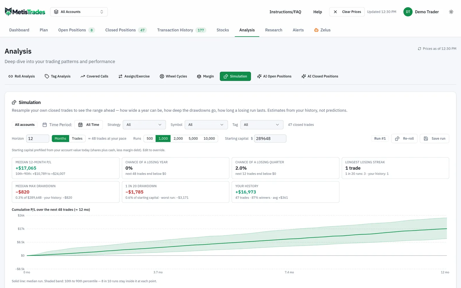
The tiles report Median 12-month P/L with its 10th–90th range, Chance of a losing year, Chance of a losing quarter, Longest losing streak (median, the 1-in-20 figure, and your actual history's longest), Median max drawdown and 1 in 20 drawdown. Two histograms show where the 12-month results and the drawdowns landed, with the worst 5% of runs in solid red. What made the difference re-runs the same simulation three ways — All trades, Without best k and Without worst k, where k is 5% of the sample — so you can see whether the whole picture rests on a few trades. In the hand example, removing trade 4 would transform every figure; that is precisely what this table measures.
Every run is seeded. The same scope, inputs and Run # always reproduce the same numbers; Re-roll advances the run number and draws a fresh set. A finished run can be kept with Save this run, which stores its inputs and headline figures (not the thousands of paths), up to 50 per user.
Plan → Risk → Simulation: random market paths over your open book
This one draws prices, not trades. It generates thousands of random market paths for the selected scope, reprices the whole open book at the end of each one, and shows the range of P/L at your horizon. Controls are Horizon (7d, 14d, 30d, 60d or Nearest exp), Paths (1,000, 2,500 or 5,000), Vol (Implied from your nearest-the-money open legs and the last VIX close, or Realized from a year of daily closes), plus Run # and Re-roll. A Chance of losing more than $… field reports the share of paths worse than any dollar figure you type.
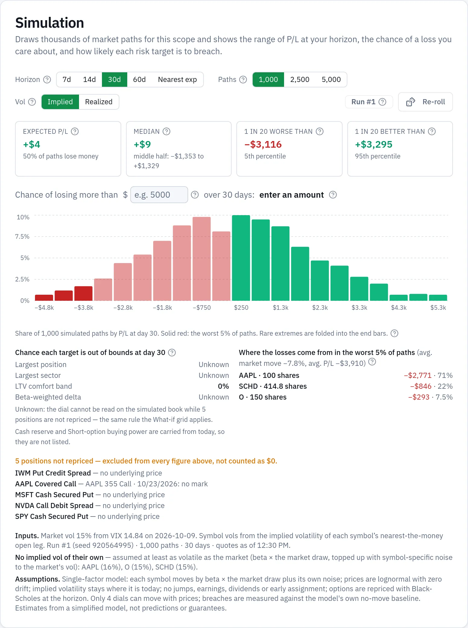
Under the hood it is a single-factor model: the market draws one lognormal return for the horizon, every symbol moves by its beta times that return plus its own noise, and options are repriced with Black-Scholes at today's implied volatility with the horizon's days elapsed. Prices are lognormal with zero drift. Positions that cannot be repriced — no cached mark, no usable implied volatility, an expired leg awaiting its close, futures and futures options — are listed under the card with the reason and excluded from every figure rather than counted as $0. The card is for Pro accounts.
Results include Expected P/L (the average across paths, with the share that lose money), Median with the 25th–75th percentile beneath it, 1 in 20 worse than and 1 in 20 better than, a histogram, the chance each price-sensitive risk target is out of bounds at the horizon, and a breakdown of where the losses come from in the worst 5% of paths.
Show range on Plan → Income, Plan → Margin and Plan → Retirement
The Plan pages each carry a deterministic projection — one line under your saved assumptions. The Show range switch, off by default, replays that same projection over many simulated paths and shades the 10th to 90th percentile behind it, with a thin median line. Turning it on adds exactly one new assumption, a volatility field starting at 16%; the projection line itself does not change.
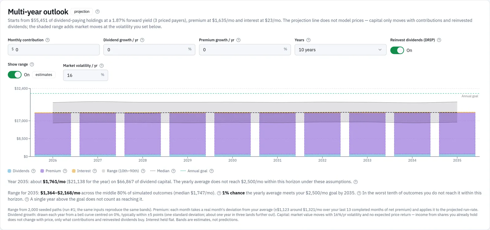
What varies differs by page. On Plan → Income, option premium is resampled from your own last 3 to 36 completed months of net premium, dividend growth is drawn each year from a bell curve centred on your rate with a 5-point standard deviation, and dividend capital moves with a market return drawn at your volatility with no expected price return. On Plan → Margin, the portfolio return is drawn at your volatility centred on your saved annual return, and the dividend yield is varied by ±10% of itself; the summary reports payoff months rather than a dollar band. On Plan → Retirement, price return, premium and dividend growth all vary, and the summary reports the share of outcomes that stay funded through the horizon plus the depletion years for the outcomes that run out. All three runs are seeded and computed in the background. These Plan pages require Pro access.
How to read the results
Median is not average. The median is the middle outcome: half the runs are better, half worse. The average is pulled by extremes. Your hand example shows the difference in miniature — the median run total was 407.5 (halfway between the fifth and sixth of the ten sorted totals, 315 and 500) while the average was only 165.5, because the −910 and −310 runs dragged the mean down. Plan → Risk → Simulation reports both: Expected P/L is the average, Median is the middle path.
The band is where most outcomes sit, not a worst case. A 10th–90th percentile band holds 8 runs in 10. One in ten lands below the bottom edge and one in ten above the top. It is not a floor.
"1 in 20" figures are tail markers. The 95th-percentile drawdown is the fall that 1 run in 20 exceeds. It is a reasonable planning number for "a bad but not unimaginable stretch" — not the worst thing that can happen.
Chance of a loss is a count, not a verdict. "40% of runs lost money" means 4 in 10 of the simulated futures finished below zero under the inputs given. It does not mean your next five trades have a 40% chance of losing; it means a strategy with your historical pattern produces losing stretches that often.
Seeded runs make results repeatable. Both Simulation tabs fix the draws to a run number, so the same scope, inputs and Run # reproduce the same figures. Re-roll draws a fresh set. If medians swing a lot between rolls, that is sampling noise: raise the run count, or read it as a sign that a few outliers dominate the sample and check the What made the difference table.
More runs means steadier percentiles, not better predictions. Going from 1,000 to 10,000 runs narrows the wobble in the output; it does not make the model more right about the world.
What the numbers do not mean. A bootstrap only knows the trades you gave it: it assumes your future trades resemble your past ones in strategy, size and market, and that each trade is independent of the one before. A price model only knows its own assumptions: zero drift, constant volatility, one market factor, no jumps, no earnings moves, no early assignment. Positions that could not be repriced are excluded, never valued at zero — so a Plan → Risk figure describes the part of your book the model could price. All of it is an estimate from a simplified model, not a prediction.
Common mistakes
- Reading the median as the expected result. Half the outcomes are worse, and the worse half is usually the longer tail. Fix: always quote the median with its 10th–90th band and the 1-in-20 drawdown beside it.
- Simulating from too few trades. A sample of a dozen outcomes just replays the same few numbers and makes the range look far more certain than it is. Fix: widen the period, drop the strategy or symbol filter, or use All accounts — MetisTrades refuses to simulate under 30 closed trades for this reason.
- Counting each leg of a roll as a separate trade. It splits one decision into several small results and hides the real size of a bad outcome. Fix: treat a whole roll chain as one trade, which is what the Closed Positions definition behind Analysis → Simulation already does.
- Re-rolling until the numbers look good. The run number changes the draw, not the book. Fix: pick a run count, note the Run # and seed, and compare runs at the same settings.
- Using the trade bootstrap to answer a market question. Analysis → Simulation never prices your open positions. Fix: use Plan → Risk → Simulation for "what could my current book do by expiration", and the bootstrap for "what could my trading pattern do over the next year".
- Ignoring the excluded-positions list. A tail figure that quietly leaves out your futures positions or an unpriced leg is not describing your whole book. Fix: read the list under the card, refresh quotes where that is the reason, and discount the result accordingly.
- Treating a probability band as a plan. "90% of outcomes stay funded" is the output of a model with fixed spending, fixed inflation and independent monthly returns. Fix: change one lever at a time — spending, date, contributions — and watch the funded share move, rather than trusting any single percentage.
Related guides and help pages
Related guides
- Plan, Track, Optimize: a complete tour of MetisTrades
- How much capital does $1,000 a month in options income take?
- Simulating the range of results ahead from your own closed trades
- Setting and Tracking an Options Income Goal
- Planning a Margin Paydown: Setting a Destination LTV and Tracking Progress
- Planning retirement income from an options portfolio